Visualización de funciones en 3D#
Ultima modificación: Feb 01, 2024 | YouTube
[1]:
import matplotlib

matplotlib.__version__
[1]:
'3.7.1'
Función de Rosenbrock#
La función de Rosenbrock de dos dimensiones se define como:
f(x, y) = 100 \cdot (x^2 - y)^2 + (1 - x)^2
para:
x \in [-2.048, 2.048]
y \in [-1.000, 4.000]
y
f(1, 1) = 0
[2]:
def f(x, y):
    return 100 * (x**2 - y) ** 2 + (1 - x) ** 2
Proceso de visualización#
Se define una malla fina en el plano X-Y.
Se computa la función z = f(x,y) para cada punto del plano.
Se visualiza z.
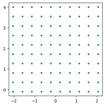
Creación de la malla#
[3]:
import numpy as np

#
# Generación de un vector de puntos para x
#
X = np.linspace(start=-2.048, stop=2.048, num=10)
X.round(3)
[3]:
array([-2.048, -1.593, -1.138, -0.683, -0.228,  0.228,  0.683,  1.138,
        1.593,  2.048])
[4]:
#
# Generación de un vector de puntos para y
#
Y = np.linspace(start=-0.1, stop=4.0, num=10)
Y.round(3)
[4]:
array([-0.1  ,  0.356,  0.811,  1.267,  1.722,  2.178,  2.633,  3.089,
        3.544,  4.   ])
[5]:
#
# Generación de una matriz para representar
# una malla de puntos
#
X, Y = np.meshgrid(X, Y)
X.round(3)
[5]:
array([[-2.048, -1.593, -1.138, -0.683, -0.228,  0.228,  0.683,  1.138,
         1.593,  2.048],
       [-2.048, -1.593, -1.138, -0.683, -0.228,  0.228,  0.683,  1.138,
         1.593,  2.048],
       [-2.048, -1.593, -1.138, -0.683, -0.228,  0.228,  0.683,  1.138,
         1.593,  2.048],
       [-2.048, -1.593, -1.138, -0.683, -0.228,  0.228,  0.683,  1.138,
         1.593,  2.048],
       [-2.048, -1.593, -1.138, -0.683, -0.228,  0.228,  0.683,  1.138,
         1.593,  2.048],
       [-2.048, -1.593, -1.138, -0.683, -0.228,  0.228,  0.683,  1.138,
         1.593,  2.048],
       [-2.048, -1.593, -1.138, -0.683, -0.228,  0.228,  0.683,  1.138,
         1.593,  2.048],
       [-2.048, -1.593, -1.138, -0.683, -0.228,  0.228,  0.683,  1.138,
         1.593,  2.048],
       [-2.048, -1.593, -1.138, -0.683, -0.228,  0.228,  0.683,  1.138,
         1.593,  2.048],
       [-2.048, -1.593, -1.138, -0.683, -0.228,  0.228,  0.683,  1.138,
         1.593,  2.048]])
[6]:
Y.round(3)
[6]:
array([[-0.1  , -0.1  , -0.1  , -0.1  , -0.1  , -0.1  , -0.1  , -0.1  ,
        -0.1  , -0.1  ],
       [ 0.356,  0.356,  0.356,  0.356,  0.356,  0.356,  0.356,  0.356,
         0.356,  0.356],
       [ 0.811,  0.811,  0.811,  0.811,  0.811,  0.811,  0.811,  0.811,
         0.811,  0.811],
       [ 1.267,  1.267,  1.267,  1.267,  1.267,  1.267,  1.267,  1.267,
         1.267,  1.267],
       [ 1.722,  1.722,  1.722,  1.722,  1.722,  1.722,  1.722,  1.722,
         1.722,  1.722],
       [ 2.178,  2.178,  2.178,  2.178,  2.178,  2.178,  2.178,  2.178,
         2.178,  2.178],
       [ 2.633,  2.633,  2.633,  2.633,  2.633,  2.633,  2.633,  2.633,
         2.633,  2.633],
       [ 3.089,  3.089,  3.089,  3.089,  3.089,  3.089,  3.089,  3.089,
         3.089,  3.089],
       [ 3.544,  3.544,  3.544,  3.544,  3.544,  3.544,  3.544,  3.544,
         3.544,  3.544],
       [ 4.   ,  4.   ,  4.   ,  4.   ,  4.   ,  4.   ,  4.   ,  4.   ,
         4.   ,  4.   ]])
[7]:
import matplotlib.pyplot as plt

plt.figure(figsize=(4, 4))
plt.scatter(X, Y, s=10)
plt.show()
Evaluación de la función (x, y)#
[8]:
#
# Generación de una matriz con los valores de f(x, y)
#
Z = f(X, Y)
Z.round(1)
[8]:
array([[1.8534e+03, 7.0230e+02, 1.9900e+02, 3.4900e+01, 3.8000e+00,
        2.9000e+00, 3.2100e+01, 1.9450e+02, 6.9590e+02, 1.8452e+03],
       [1.4829e+03, 4.8270e+02, 9.2700e+01, 4.1000e+00, 1.0700e+01,
        9.8000e+00, 1.3000e+00, 8.8200e+01, 4.7640e+02, 1.4747e+03],
       [1.1539e+03, 3.0470e+02, 2.7900e+01, 1.4700e+01, 5.9200e+01,
        5.8300e+01, 1.2000e+01, 2.3400e+01, 2.9830e+02, 1.1457e+03],
       [8.6640e+02, 1.6820e+02, 4.6000e+00, 6.6900e+01, 1.4910e+02,
        1.4820e+02, 6.4200e+01, 1.0000e-01, 1.6180e+02, 8.5820e+02],
       [6.2040e+02, 7.3200e+01, 2.2900e+01, 1.6060e+02, 2.8050e+02,
        2.7960e+02, 1.5790e+02, 1.8300e+01, 6.6800e+01, 6.1220e+02],
       [4.1590e+02, 1.9600e+01, 8.2600e+01, 2.9580e+02, 4.5350e+02,
        4.5260e+02, 2.9310e+02, 7.8000e+01, 1.3300e+01, 4.0770e+02],
       [2.5300e+02, 7.6000e+00, 1.8380e+02, 4.7260e+02, 6.6790e+02,
        6.6700e+02, 4.6980e+02, 1.7930e+02, 1.3000e+00, 2.4480e+02],
       [1.3150e+02, 3.7100e+01, 3.2650e+02, 6.9080e+02, 9.2390e+02,
        9.2300e+02, 6.8800e+02, 3.2200e+02, 3.0800e+01, 1.2330e+02],
       [5.1500e+01, 1.0820e+02, 5.1080e+02, 9.5050e+02, 1.2214e+03,
        1.2205e+03, 9.4780e+02, 5.0620e+02, 1.0180e+02, 4.3300e+01],
       [1.3100e+01, 2.2070e+02, 7.3650e+02, 1.2517e+03, 1.5603e+03,
        1.5594e+03, 1.2490e+03, 7.3200e+02, 2.1430e+02, 4.9000e+00]])
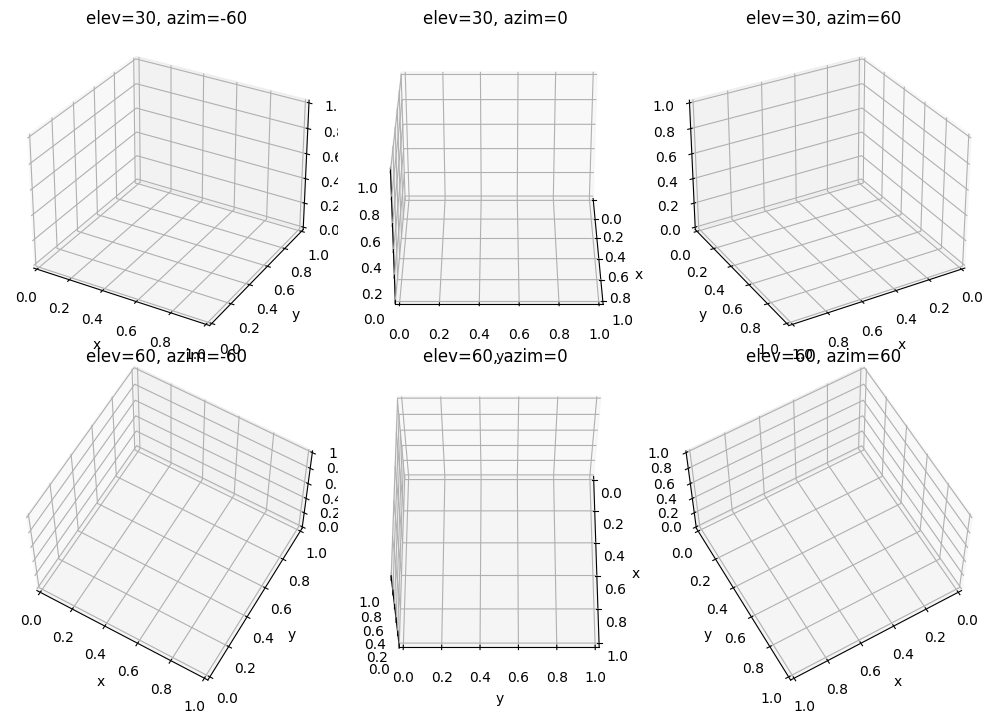
Projection 3d#
[9]:
fig = plt.figure(figsize=(10, 7))

i = 1
for elev in [30, 60]:
    for azim in [-60, 0, 60]:

        ax = fig.add_subplot(2, 3, i, projection="3d", azim=azim, elev=elev)
        i += 1
        plt.xlabel("x")
        plt.ylabel("y")
        plt.title("elev={}, azim={}".format(elev, azim))

plt.tight_layout()
plt.show()
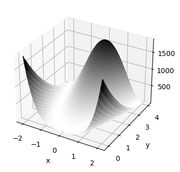
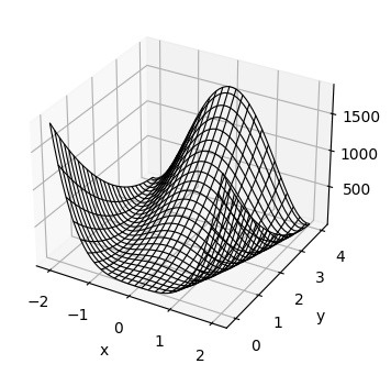
plot_surface()#
[10]:
#
# Gráfica de la función
#
from matplotlib import cm

X = np.linspace(start=-2.048, stop=2.048, num=50)
Y = np.linspace(start=-0.1, stop=4.0, num=50)
X, Y = np.meshgrid(X, Y)
Z = f(X, Y)

ax = plt.figure(figsize=(4, 4)).add_subplot(projection="3d")
ax.plot_surface(
    X,
    Y,
    Z,
    cmap=cm.binary,
    linewidth=1,
    antialiased=False,
)

plt.xlabel("x")
plt.ylabel("y")
plt.show()
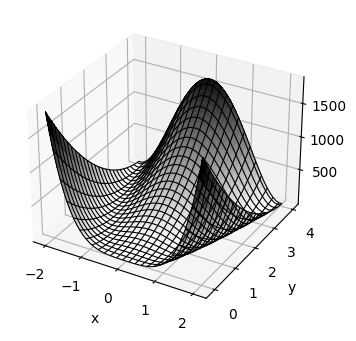
plot_wireframe()#
[11]:
ax = plt.figure(figsize=(4, 4)).add_subplot(projection="3d")
ax.plot_wireframe(
    X,
    Y,
    Z,
    color="black",
    linewidth=0.8,
    alpha=1.0,
    rstride=2,
    cstride=2,
)
plt.xlabel("x")
plt.ylabel("y")
plt.show()
Combinación de plot_wireframe() y plot.suface() para mejorar la visualización#
[12]:
ax = plt.figure(figsize=(4, 4)).add_subplot(projection="3d")

ax.plot_surface(
    X,
    Y,
    Z,
    cmap=cm.binary,
    linewidth=1,
    antialiased=False,
)

ax.plot_wireframe(
    X,
    Y,
    Z,
    color="black",
    linewidth=0.8,
    alpha=1.0,
    rstride=2,
    cstride=2,
)

plt.xlabel("x")
plt.ylabel("y")
plt.show()
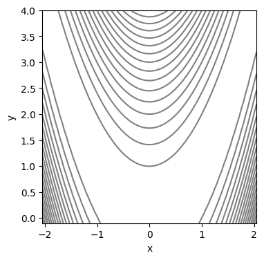
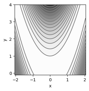
plt.contour()#
[13]:
#
# Líneas de nivel con el mismo color
#
fig = plt.figure(figsize=(4, 4))

plt.gca().contour(
    X,
    Y,
    Z,
    colors="gray",
    levels=20,
)

plt.xlabel("x")
plt.ylabel("y")
plt.show()
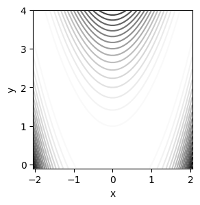
[14]:
#
# Líneas de nivel con diferentes colores
#
fig = plt.figure(figsize=(3, 3))
plt.gca().contour(
    X,
    Y,
    Z,
    cmap=cm.Greys,
    levels=20,
)

plt.xlabel("x")
plt.ylabel("y")
plt.show()
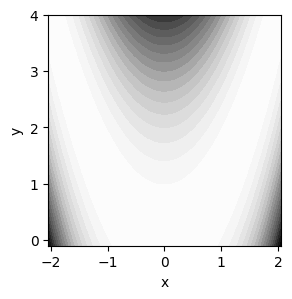
plt.contourf()#
[15]:
fig = plt.figure(figsize=(3, 3))

plt.gca().contourf(
    X,
    Y,
    Z,
    cmap=cm.Greys,
    levels=20,
)

plt.xlabel("x")
plt.ylabel("y")
plt.show()
Uso de contour() y contourf() para mejorar la visualización#
[16]:
fig = plt.figure(figsize=(3, 3))

plt.gca().contourf(
    X,
    Y,
    Z,
    cmap=cm.Greys,
    levels=20,
    alpha=1.0,
)

plt.gca().contour(
    X,
    Y,
    Z,
    colors="gray",
    levels=20,
)


plt.xlabel("x")
plt.ylabel("y")
plt.show()
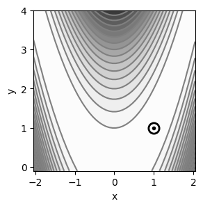
Punto de mínima de la función#
[17]:
fig = plt.figure(figsize=(3, 3))

plt.gca().contourf(
    X,
    Y,
    Z,
    cmap=cm.Greys,
    levels=20,
    alpha=1.0,
)

plt.gca().contour(
    X,
    Y,
    Z,
    colors="gray",
    levels=20,
)

plt.plot(
    [1],
    [1],
    "o",
    color="black",
    fillstyle="none",
    markersize=11,
    markeredgewidth=2,
)

plt.plot(
    [1],
    [1],
    ".",
    color="black",
)

plt.xlabel("x")
plt.ylabel("y")
plt.show()