El método del gradiente descendente#
Ultima modificación: Feb 01, 2024 | YouTube
Método del gradiente descendente#
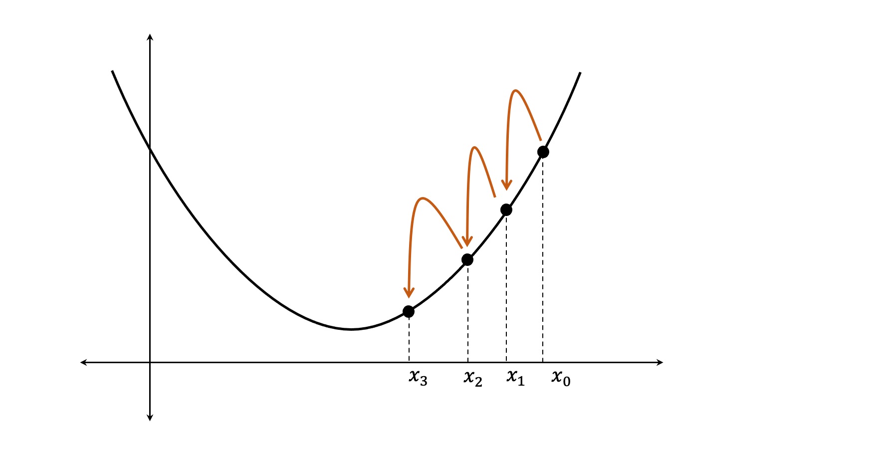
Es un proceso iterativo en que el valor actual de x se corrige sumandole un valor \Delta x con signo contrario a la derivada (dirección de descenso), hasta alcanzar el punto de mínima.
La ecuación de corrección o mejora es:
x_k = x_{k-1} - \mu \frac{d}{dx} f(x_{k-1})
donde \mu es la tasa o factor de aprendizaje.
Notación vectorial:
\mathbf{w}_k = \mathbf{w}_{k-1} - \mu \frac{\partial}{\partial \mathbf{w}} f(\mathbf{w}_{k-1})
Función de Rosenbrock#
La función de Rosenbrock de dos dimensiones se define como:
f(x, y) = 100 \cdot (x^2 - y)^2 + (1 - x)^2
para:
x \in [-2.048, 2.048]
y \in [-1.000, 4.000]
y
f(1, 1) = 0
.
Derivada de f(x, y) respecto a x#
\begin{split} \frac{\partial}{\partial x} f(x, y) & = \frac{\partial}{\partial x} \left[ 100 (x^2 - y)^2 + (1-x)^2 \right] \\ \\ & = \frac{\partial}{\partial x} \left[ 100 (x^2 - y)^2 \right] + \frac{\partial}{\partial x} \left[ (1-x)^2 \right] \\ \\ & = 100 \cdot 2 \cdot (x^2 - y) \frac{\partial}{\partial x} (x^2 - y) + 2 \cdot (1 - x)\frac{\partial}{\partial x} (1-x) \\ \\ & = 100 \cdot 2 \cdot (x^2 - y) \frac{\partial}{\partial x} (x^2) + 2 \cdot (1 - x)\frac{\partial}{\partial x} (-x) \\ \\ & = 200 \cdot (x^2 - y) \cdot 2x + 2 \cdot (1 - x) \cdot (-1) \\ \\ & = 400 x (x^2 - y) - 2 (1- x) \end{split}
Derivada de f(x, y) respecto a y#
\begin{split} \frac{\partial}{\partial y} f(x, y) & = \frac{\partial}{\partial y} \left[ 100 (x^2 - y)^2 + (1-x)^2 \right] \\ \\ & = \frac{\partial}{\partial y} \left[ 100 (x^2 - y)^2 \right] + \frac{\partial}{\partial y} \left[ (1-x)^2 \right] \\ \\ & = 100 \cdot 2 \cdot (x^2 - y) \frac{\partial}{\partial y} (x^2 - y) + 2 \cdot (1 - x)\frac{\partial}{\partial y} (1-x) \\ \\ & = -200 \cdot (x^2 - y) \frac{\partial}{\partial y} (-y) + 2 \cdot (1 - x) \cdot 0 \\ \\ & = -200 \cdot (x^2 - y) \end{split}
Gradiente algebraico#
El gradiente expresado en forma matricial sería:
g(x, y) = \frac{\partial}{\partial \mathbf{w}} f(\mathbf{w}) = \left[ \begin{array}{c} 400 x (x^2-y) - 2(1 - x) \\ -200(x^2 - y) \end{array} \right]
Ejemplo del cómputo#
[1]:
#
# Función
#
def f(x, y):
    return 100 * (x ** 2 - y) ** 2 + (1 - x) ** 2


#
# Gradiente
#
def g(x, y):
    grad_x = 400 * x * (x ** 2 - y) - 2 * (1 - x)
    grad_y = -200 * (x ** 2 - y)
    return grad_x, grad_y


#
# Función de mejora
#
def improve(x, y, mu):
    grad_x, grad_y = g(x, y)
    x = x - mu * grad_x
    y = y - mu * grad_y
    return x, y


#
# Punto de inicio
#
x = -0.5
y = +3.5

history = {"x": [x], "y": [y], "f": [f(x, y)]}


for epoch in range(50):
    x, y = improve(x, y, mu=0.001)
    history["x"].append(x)
    history["y"].append(y)
    history["f"].append(f(x, y))

#
# Ultimo resultado obtenido
#
print("      x = {:6.5f}\n      y = {:+6.5f}\nf(x, y) = {:+6.5f}".format(x, y, f(x, y)))
      x = -1.47399
      y = +2.14267
f(x, y) = +6.21043
[2]:
import matplotlib.pyplot as plt
import numpy as np
from matplotlib import cm
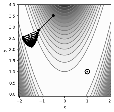
def plot_contour():
X = np.linspace(start=-2.048, stop=2.048, num=50)
Y = np.linspace(start=-0.1, stop=4.0, num=50)
X, Y = np.meshgrid(X, Y)
Z = f(X, Y)
plt.subplots(figsize=(4, 4))
plt.gca().contourf(X, Y, Z, cmap=cm.Greys, levels=20, alpha=1.0)
plt.gca().contour(X, Y, Z, colors="gray", levels=20)
plt.plot(
[1], [1], "o", color="black", fillstyle="none", markersize=11, markeredgewidth=2
)
plt.plot([1], [1], ".", color="black")
plt.xlabel("x")
plt.ylabel("y")
plot_contour()
plt.plot(history["x"], history["y"], "o-", color="k")
plt.show()
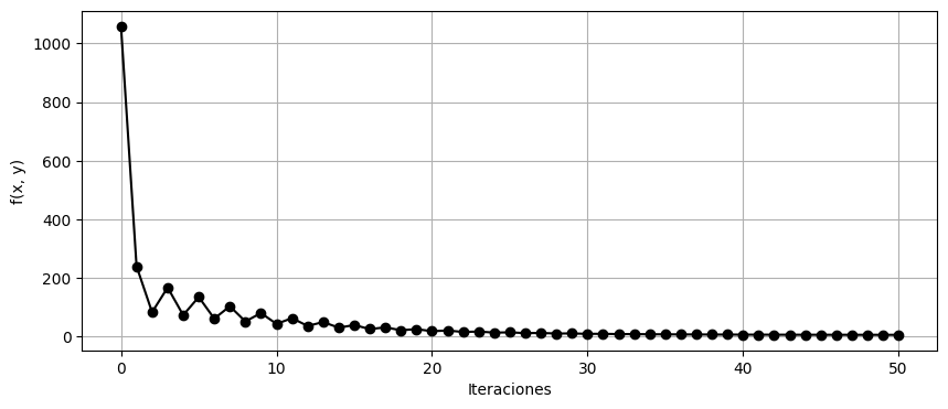
[3]:
plt.figure(figsize=(10, 4))
plt.plot(history["f"], "o-k")
plt.xlabel("Iteraciones")
plt.ylabel("f(x, y)")
plt.grid()