Manejo básico de imágenes#
Ultima modificación: Feb 04, 2024 | YouTube
[1]:
import matplotlib.pyplot as plt
import numpy as np
from PIL import Image
[2]:
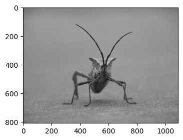
#
# Una imagen RGB PNG es representada coomo un array de 3 dimensiones que
# indican los colornes [R, G, B] de cada pixel.
#
org_img = np.asarray(Image.open("assets/stinkbug.png"))

# Dimensiones de la imagen
print(org_img.shape)

# Representación como un array de NumPy
print(repr(org_img))
(808, 1088, 3)
array([[[108, 108, 108],
        [108, 108, 108],
        [108, 108, 108],
        ...,
        [112, 112, 112],
        [112, 112, 112],
        [112, 112, 112]],

       [[108, 108, 108],
        [108, 108, 108],
        [108, 108, 108],
        ...,
        [113, 113, 113],
        [113, 113, 113],
        [112, 112, 112]],

       [[108, 108, 108],
        [108, 108, 108],
        [108, 108, 108],
        ...,
        [113, 113, 113],
        [113, 113, 113],
        [112, 112, 112]],

       ...,

       [[108, 108, 108],
        [109, 109, 109],
        [109, 109, 109],
        ...,
        [116, 116, 116],
        [116, 116, 116],
        [116, 116, 116]],

       [[108, 108, 108],
        [108, 108, 108],
        [109, 109, 109],
        ...,
        [116, 116, 116],
        [116, 116, 116],
        [116, 116, 116]],

       [[108, 108, 108],
        [108, 108, 108],
        [108, 108, 108],
        ...,
        [116, 116, 116],
        [116, 116, 116],
        [116, 116, 116]]], dtype=uint8)
[3]:
org_img.shape
[3]:
(808, 1088, 3)
[4]:
plt.figure(figsize=(4, 4))
plt.imshow(org_img)
plt.show()
[5]:
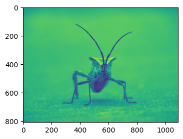
#
# Aplicación de un seudocolor para mejorar el contraste
#
lum_img = org_img[:, :, 0]
lum_img
[5]:
array([[108, 108, 108, ..., 112, 112, 112],
       [108, 108, 108, ..., 113, 113, 112],
       [108, 108, 108, ..., 113, 113, 112],
       ...,
       [108, 109, 109, ..., 116, 116, 116],
       [108, 108, 109, ..., 116, 116, 116],
       [108, 108, 108, ..., 116, 116, 116]], dtype=uint8)
[6]:
plt.figure(figsize=(4, 4))
plt.imshow(lum_img)
plt.show()
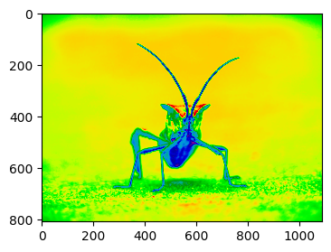
[7]:
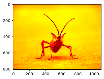
#
# Aplicación de una luminosidad
#
plt.figure(figsize=(4, 4))
plt.imshow(lum_img, cmap="hot")
plt.show()
[8]:
#
# Cambio de colormap de un objeto existente
#
plt.figure(figsize=(4, 4))
plt.imshow(lum_img).set_cmap("nipy_spectral")
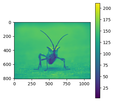
[9]:
#
# Escala de color de referencia
#
plt.figure(figsize=(4, 4))
plt.imshow(lum_img)
plt.colorbar()
plt.show()
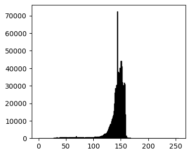
[10]:
#
# Examinación de un rango de datos
#
plt.figure(figsize=(4, 3.5))
plt.hist(lum_img.ravel(), bins=range(256), fc="k", ec="k")
plt.show()
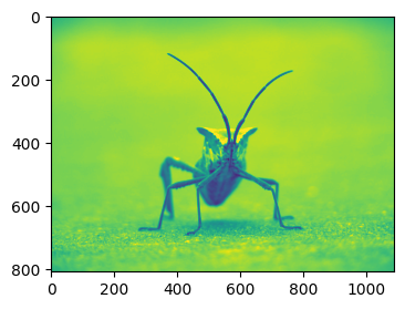
[11]:
#
# Se resalta la información del rango del pico
#
plt.figure(figsize=(4, 4))
plt.imshow(lum_img, clim=(0, 175))
plt.show()

[12]:
#
# Esta misma tarea puede ser realizada con set_clim()
#
plt.figure(figsize=(4, 4))
plt.imshow(lum_img).set_clim(0, 175)
plt.show()
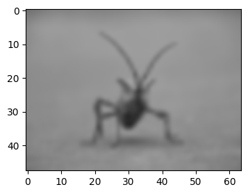
[13]:
#
# Redimensionamiento de la imagen e interpolacion (nearest)
#
plt.figure(figsize=(4, 4))
org_img = Image.open("assets/stinkbug.png")
org_img.thumbnail((64, 64))
plt.imshow(org_img)
plt.show()

[14]:
#
# Interpolación bilineal
#
plt.figure(figsize=(4, 4))
plt.imshow(org_img, interpolation="bilinear")
plt.show()

[15]:
#
# Interpolación bicubica
#
plt.figure(figsize=(4, 4))
plt.imshow(org_img, interpolation="bicubic")
plt.show()