Mallas de gráficas#
0:00 min | Última modificación: Octubre 13, 2021 | [YouTube]
[1]:
import matplotlib.pyplot as plt
import numpy as np
import seaborn as sns
[2]:
tips = sns.load_dataset("tips")
penguins = sns.load_dataset("penguins")
[3]:
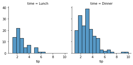
#
# FacetGrid() define las columnas
#
g = sns.FacetGrid(tips, col="time",)

g.map(sns.histplot, "tip",)

plt.show()
[4]:
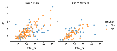
#
# Adición de la legenda
#
g = sns.FacetGrid(tips, col="sex", hue="smoker",)

g.map(sns.scatterplot, "total_bill", "tip", alpha=.7,)

g.add_legend()

plt.show()
[5]:
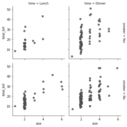
#
# Adición de titulos al margen
#
g = sns.FacetGrid(tips, row="smoker", col="time", margin_titles=True,)

g.map(sns.regplot, "size", "total_bill", color=".3", fit_reg=False, x_jitter=.1,)

plt.show()
[6]:
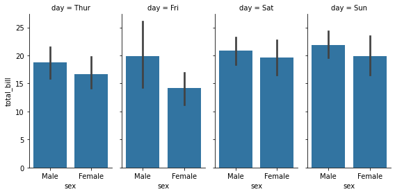
#
# Modificación del parámetro aspecto de la
# gráfica
#
g = sns.FacetGrid(tips, col="day", height=4, aspect=.5,)

g.map(sns.barplot, "sex", "total_bill", order=["Male", "Female"],)

plt.show()
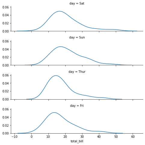
[7]:
#
# Ordenamiento de la secuencia de figuras
#
ordered_days = tips.day.value_counts().index

g = sns.FacetGrid(tips, row="day", row_order=ordered_days,
                  height=1.7, aspect=4,)

g.map(sns.kdeplot, "total_bill")

plt.show()
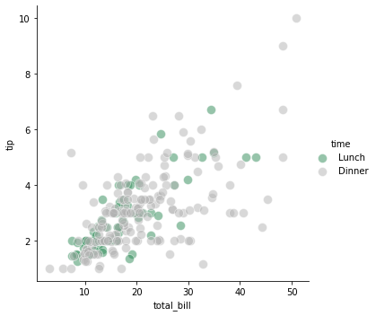
[8]:
#
# Paleta de colores
#
pal = dict(Lunch="seagreen", Dinner=".7",)

g = sns.FacetGrid(tips, hue="time", palette=pal, height=5,)

g.map(sns.scatterplot, "total_bill", "tip", s=100, alpha=.5, )

g.add_legend()

plt.show()
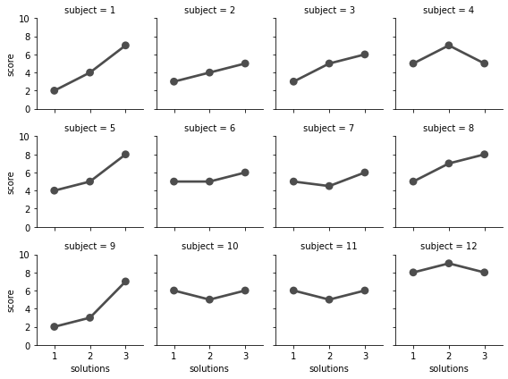
[9]:
attend = sns.load_dataset("attention").query("subject <= 12")

g = sns.FacetGrid(attend, col="subject", col_wrap=4, height=2, ylim=(0, 10), )

g.map(sns.pointplot, "solutions", "score", order=[1, 2, 3], color=".3", ci=None,)

plt.show()
[ ]:
#
# Gráfico usando pairplot()
#
sns.pairplot(penguins)
plt.show()
[ ]:
#
# Uso de PairGrid() para especificar el tipo de
# gráfico en cada parte
#
g = sns.PairGrid(penguins)
g.map_upper(sns.histplot)
g.map_lower(sns.kdeplot, fill=True)
g.map_diag(sns.histplot, kde=True)
plt.show()